(Solved): Please ii-) Fig. 1.16. The incidence graph of the Fano plane: the Heawood graph the edge ...

Please ii-)

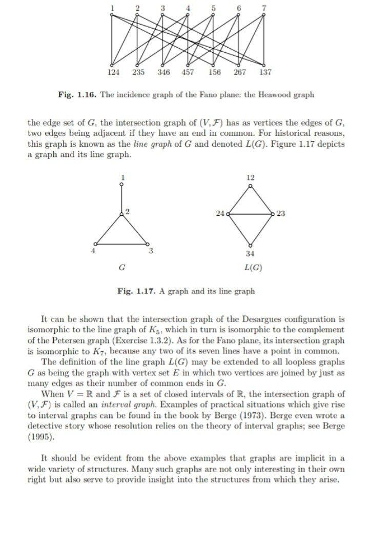
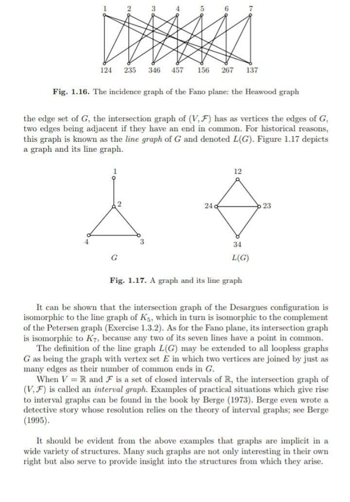
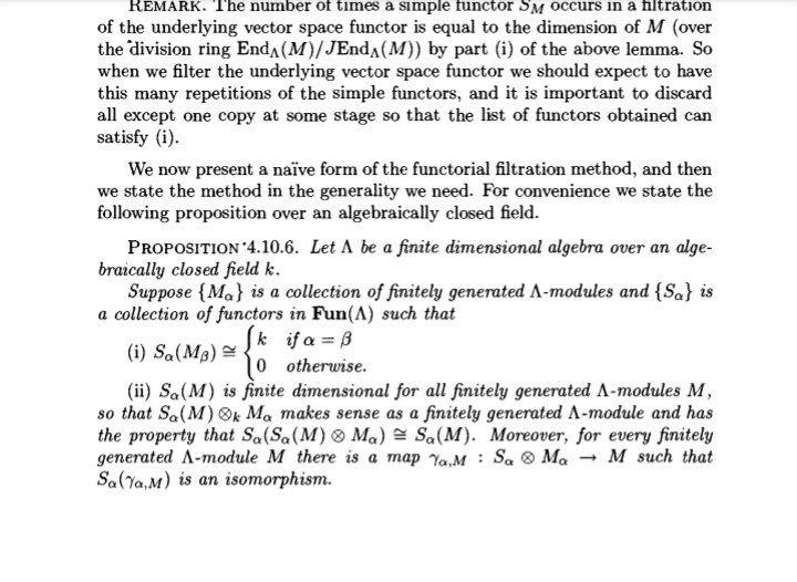
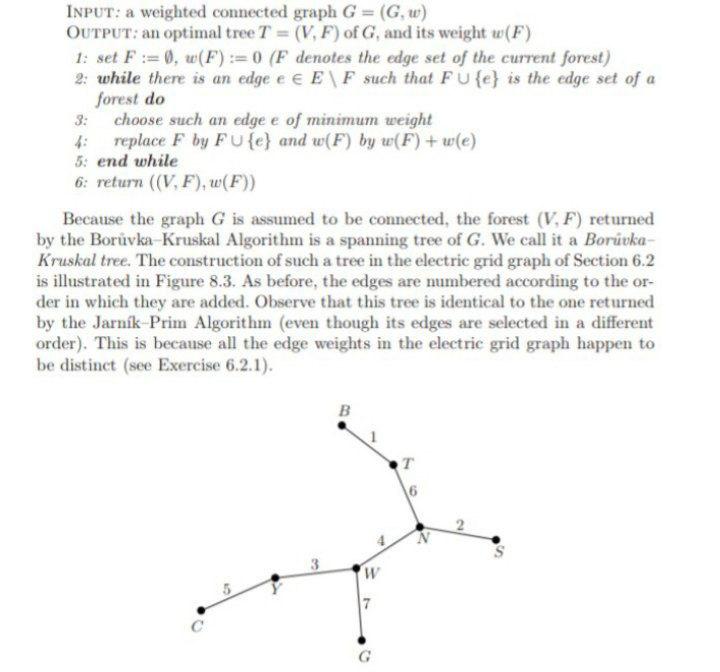
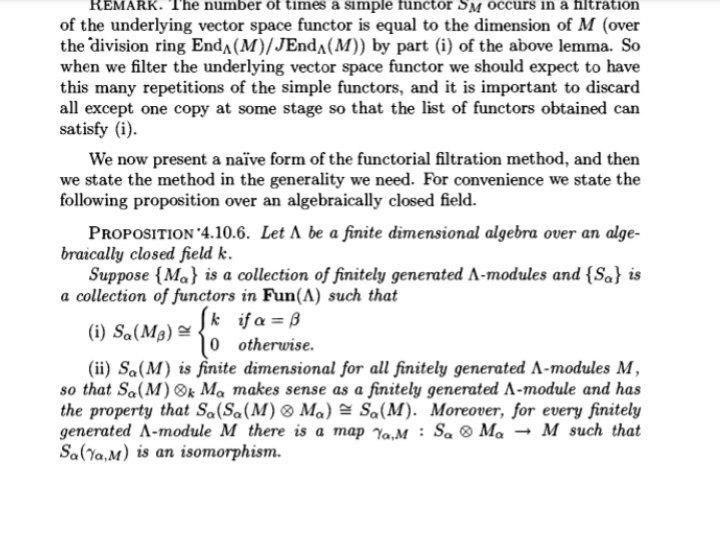
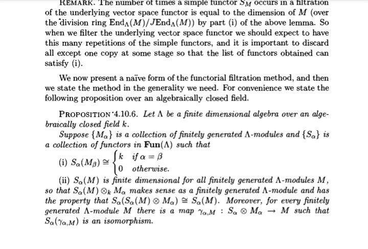
Fig. 1.16. The incidence graph of the Fano plane: the Heawood graph the edge set of \( G \), the intersection graph of \( (V, \mathcal{F}) \) has as vertices the edges of \( G \), two edges being adjacent if they have an end in common. For historical reasons, this graph is known as the line graph of \( G \) and denoted \( L(G) \). Figure \( 1.17 \) depicts a graph and its line graph. Fig. 1.17. A graph and its line graph It can be shown that the intersection graph of the Desargues configuration is isomorphic to the line graph of \( K_{5} \), which in turn is isomorphic to the complement of the Petersen graph (Exercise 1.3.2). As for the Fano plane, its intersection graph is isomorphic to \( K_{7} \), because any two of its seven lines have a point in common. The definition of the line graph \( L(G) \) may be extended to all loopless graphs \( G \) as being the graph with vertex set \( E \) in which two vertices are joined by just as many edges as their number of common ends in \( G \). When \( V=\mathbb{R} \) and \( \mathcal{F} \) is a set of closed intervals of \( \mathbb{R} \), the intersection graph of \( (V, \mathcal{F}) \) is called an interval graph. Examples of practical situations which give rise to interval graphs can be found in the book by Berge (1973). Berge even wrote a detective story whose resolution relies on the theory of interval graphs; see Berge (1995). It should be evident from the above examples that graphs are implicit in a wide variety of structures. Many such graphs are not only interesting in their own right but also serve to provide insight into the structures from which they arise. Fig. 1.16. The incidence graph of the Fano plane: the Heawood graph the edge set of \( G \), the intersection graph of \( (V, \mathcal{F}) \) has as vertices the edges of \( G \), two edges being adjacent if they have an end in common. For historical reasons, this graph is known as the line graph of \( G \) and denoted \( L(G) \). Figure \( 1.17 \) depicts a graph and its line graph. Fig. 1.17. A graph and its line graph It can be shown that the intersection graph of the Desargues configuration is isomorphic to the line graph of \( K_{5} \), which in turn is isomorphic to the complement of the Petersen graph (Exercise 1.3.2). As for the Fano plane, its intersection graph is isomorphic to \( K_{7} \), because any two of its seven lines have a point in common. The definition of the line graph \( L(G) \) may be extended to all loopless graphs \( G \) as being the graph with vertex set \( E \) in which two vertices are joined by just as many edges as their number of common ends in \( G \). When \( V=\mathbb{R} \) and \( \mathcal{F} \) is a set of closed intervals of \( \mathbb{R} \), the intersection graph of \( (V, \mathcal{F}) \) is called an interval graph. Examples of practical situations which give rise to interval graphs can be found in the book by Berge (1973). Berge even wrote a detective story whose resolution relies on the theory of interval graphs; see Berge (1995). It should be evident from the above examples that graphs are implicit in a wide variety of structures. Many such graphs are not only interesting in their own right but also serve to provide insight into the structures from which they arise. REMARK. The number of times a simple functor \( S_{M} \) occurs in a filtration of the underlying vector space functor is equal to the dimension of \( M \) (over the division ring \( \operatorname{End}_{\Lambda}(M) / J \operatorname{End}_{\Lambda}(M) \) ) by part (i) of the above lemma. So when we filter the underlying vector space functor we should expect to have this many repetitions of the simple functors, and it is important to discard all except one copy at some stage so that the list of functors obtained can satisfy (i). We now present a naïe form of the functorial filtration method, and then we state the method in the generality we need. For convenience we state the following proposition over an algebraically closed field. Proposition 4 4.10.6. Let \( \Lambda \) be a finite dimensional algebra over an algebraically closed field \( k \). Suppose \( \left\{M_{\alpha}\right\} \) is a collection of finitely generated \( \Lambda \)-modules and \( \left\{S_{\alpha}\right\} \) is a collection of functors in Fun( \( \Lambda \) ) such that (i) \( S_{\alpha}\left(M_{\beta}\right) \cong\left\{\begin{array}{ll}k & \text { if } \alpha=\beta \\ 0 & \text { otherwise. }\end{array}\right. \) (ii) \( S_{\alpha}(M) \) is finite dimensional for all finitely generated \( \Lambda \)-modules \( M \), so that \( S_{\alpha}(M) \otimes_{k} M_{\alpha} \) makes sense as a finitely generated \( \Lambda \)-module and has the property that \( S_{\alpha}\left(S_{\alpha}(M) \otimes M_{\alpha}\right) \cong S_{\alpha}(M) \). Moreover, for every finitely generated \( \Lambda \)-module \( M \) there is a map \( \gamma_{\alpha, M}: S_{\alpha} \otimes M_{\alpha} \rightarrow M \) such that \( S_{\alpha}\left(\gamma_{\alpha, M}\right) \) is an isomorphism. INPUT: a weighted connected graph \( G=(G, w) \) OUTPUT: an optimal tree \( T=(V, F) \) of \( G \), and its weight \( w(F) \) 1: set \( F:=\emptyset, w(F):=0(F \) denotes the edge set of the current forest) 2: while there is an edge \( e \in E \backslash F \) such that \( F \cup\{e\} \) is the edge set of a forest do 3: choose such an edge \( e \) of minimum weight 4: replace \( F \) by \( F \cup\{e\} \) and \( w(F) \) by \( w(F)+w(e) \) 5: end while 6: return \( ((V, F), w(F)) \) Because the graph \( G \) is assumed to be connected, the forest \( (V, F) \) returned by the Bor?vka-Kruskal Algorithm is a spanning tree of \( G \). We call it a BoruvkaKruskal tree. The construction of such a tree in the electric grid graph of Section \( 6.2 \) is illustrated in Figure 8.3. As before, the edges are numbered according to the order in which they are added. Observe that this tree is identical to the one returned by the Jarnik-Prim Algorithm (even though its edges are selected in a different order). This is because all the edge weights in the electric grid graph happen to be distinct (see Exercise 6.2.1). REMARK. The number of times a simple functor \( S_{M} \) occurs in a filtration of the underlying vector space functor is equal to the dimension of \( M \) (over the division ring \( \operatorname{End}_{\Lambda}(M) / J \operatorname{End}_{\Lambda}(M) \) ) by part (i) of the above lemma. So when we filter the underlying vector space functor we should expect to have this many repetitions of the simple functors, and it is important to discard all except one copy at some stage so that the list of functors obtained can satisfy (i). We now present a naïve form of the functorial filtration method, and then we state the method in the generality we need. For convenience we state the following proposition over an algebraically closed field. Proposition'4.10.6. Let \( \Lambda \) be a finite dimensional algebra over an algebraically closed field \( k \). Suppose \( \left\{M_{\alpha}\right\} \) is a collection of finitely generated \( \Lambda \)-modules and \( \left\{S_{\alpha}\right\} \) is a collection of functors in Fun( \( \Lambda \) ) such that (i) \( S_{\alpha}\left(M_{\beta}\right) \cong\left\{\begin{array}{ll}k & \text { if } \alpha=\beta \\ 0 & \text { otherwise. }\end{array}\right. \) (ii) \( S_{\alpha}(M) \) is finite dimensional for all finitely generated \( \Lambda \)-modules \( M \), so that \( S_{\alpha}(M) \otimes_{k} M_{\alpha} \) makes sense as a finitely generated \( \Lambda \)-module and has the property that \( S_{\alpha}\left(S_{\alpha}(M) \otimes M_{\alpha}\right) \cong S_{\alpha}(M) \). Moreover, for every finitely generated \( \Lambda \)-module \( M \) there is a map \( \gamma_{\alpha, M}: S_{\alpha} \otimes M_{\alpha} \rightarrow M \) such that \( S_{\alpha}\left(\gamma_{\alpha, M}\right) \) is an isomorphism. REMARK. The number of times a simple functor \( S_{M} \) occurs in a filtration of the underlying vector space functor is equal to the dimension of \( M \) (over the division ring End \( _{\Lambda}(M) / J \operatorname{End}_{\Lambda}(M) \) ) by part (i) of the above lemma. So when we filter the underlying vector space functor we should expect to have this many repetitions of the simple functors, and it is important to discard all except one copy at some stage so that the list of functors obtained can satisfy (i). We now present a naive form of the functorial filtration method, and then we state the method in the generality we need. For convenience we state the following proposition over an algebraically closed field. ProPosition \( 4.10 .6 \). Let \( \Lambda \) be a finite dimensional algebra over an algebraically closed field \( k \). Suppose \( \left\{M_{\alpha}\right\} \) is a collection of finitely generated \( \Lambda \)-modules and \( \left\{S_{\alpha}\right\} \) is a collection of functors in \( \mathbf{F u n}(\Lambda) \) such that (i) \( S_{\alpha}\left(M_{\beta}\right) \cong\left\{\begin{array}{ll}k & \text { if } \alpha=\beta \\ 0 & \text { otherwise. }\end{array}\right. \) (ii) \( S_{\alpha}(M) \) is finite dimensional for all finitely generated \( \Lambda \)-modules \( M \), so that \( S_{\alpha}(M) \otimes_{k} M_{\alpha} \) makes sense as a finitely generated \( \Lambda \)-module and has the property that \( S_{\alpha}\left(S_{\alpha}(M) \otimes M_{\alpha}\right) \cong S_{\alpha}(M) \). Moreover, for every finitely generated \( \Lambda \)-module \( M \) there is a map \( \gamma_{\alpha, M}: S_{\alpha} \otimes M_{\alpha} \rightarrow M \) such that \( S_{\alpha}\left(\gamma_{\alpha, M}\right) \) is an isomorphism.