(Solved): Let us now describe the motion of a double pendulum. The double pendulum is d ...

???????

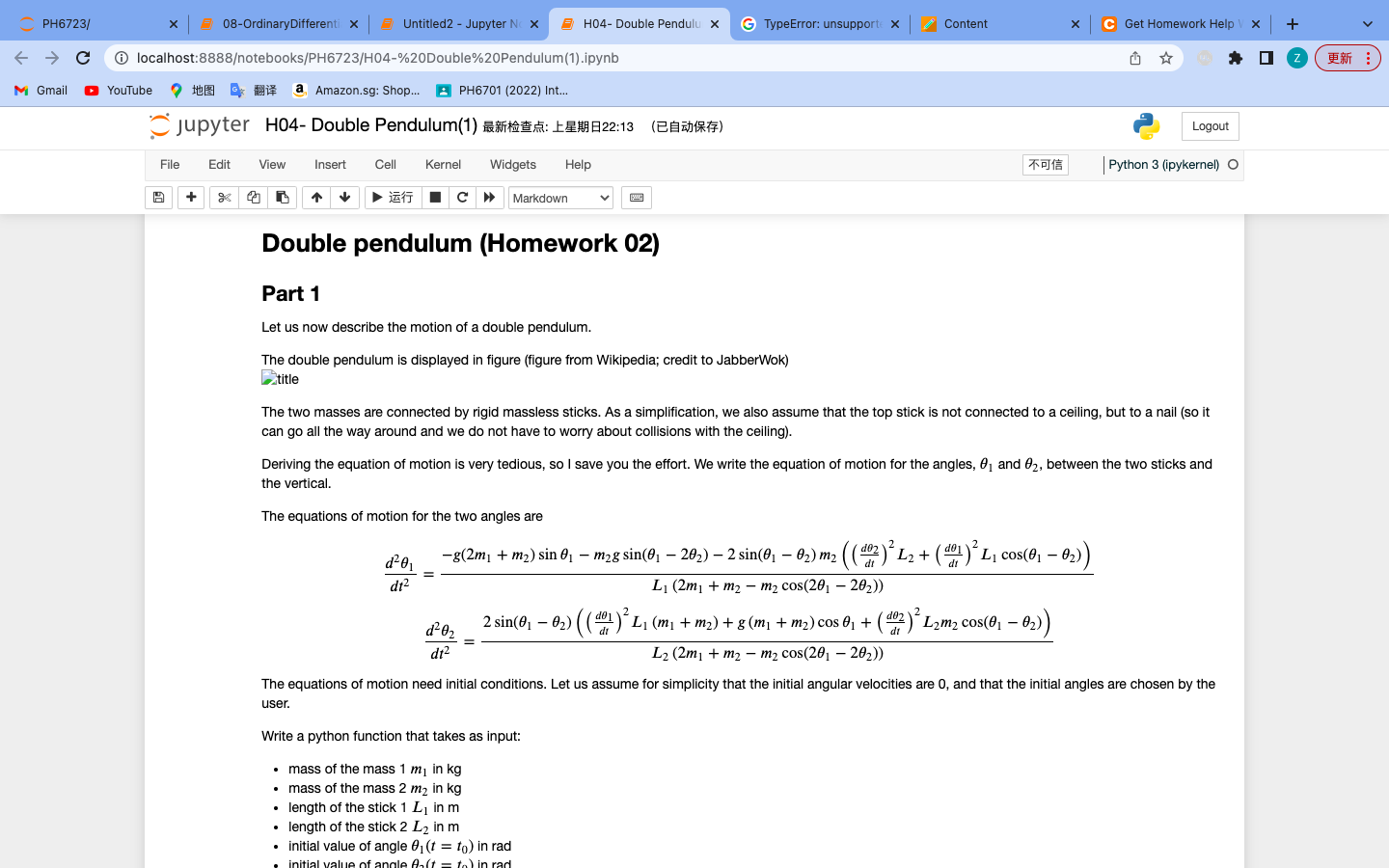
Let us now describe the motion of a double pendulum. The double pendulum is displayed in figure (figure from Wikipedia; credit to JabberWok) atitle The two masses are connected by rigid massless sticks. As a simplification, we also assume that the top stick is not connected to a ceiling, but to a nail (so it can go all the way around and we do not have to worry about collisions with the ceiling). Deriving the equation of motion is very tedious, so I save you the effort. We write the equation of motion for the angles, \( \theta_{1} \) and \( \theta_{2} \), between the two sticks and the vertical. The equations of motion for the two angles are \[ \begin{array}{c} \frac{d^{2} \theta_{1}}{d t^{2}}=\frac{-g\left(2 m_{1}+m_{2}\right) \sin \theta_{1}-m_{2} g \sin \left(\theta_{1}-2 \theta_{2}\right)-2 \sin \left(\theta_{1}-\theta_{2}\right) m_{2}\left(\left(\frac{d \theta_{2}}{d t}\right)^{2} L_{2}+\left(\frac{d \theta_{1}}{d t}\right)^{2} L_{1} \cos \left(\theta_{1}-\theta_{2}\right)\right)}{L_{1}\left(2 m_{1}+m_{2}-m_{2} \cos \left(2 \theta_{1}-2 \theta_{2}\right)\right)} \\ \frac{d^{2} \theta_{2}}{d t^{2}}=\frac{2 \sin \left(\theta_{1}-\theta_{2}\right)\left(\left(\frac{d \theta_{1}}{d t}\right)^{2} L_{1}\left(m_{1}+m_{2}\right)+g\left(m_{1}+m_{2}\right) \cos \theta_{1}+\left(\frac{d \theta_{2}}{d t}\right)^{2} L_{2} m_{2} \cos \left(\theta_{1}-\theta_{2}\right)\right)}{L_{2}\left(2 m_{1}+m_{2}-m_{2} \cos \left(2 \theta_{1}-2 \theta_{2}\right)\right)} \end{array} \] The equations of motion need initial conditions. Let us assume for simplicity that the initial angular velocities are 0 , and that the initial angles are chosen by the user. 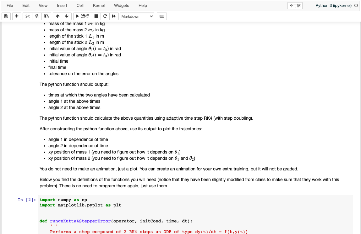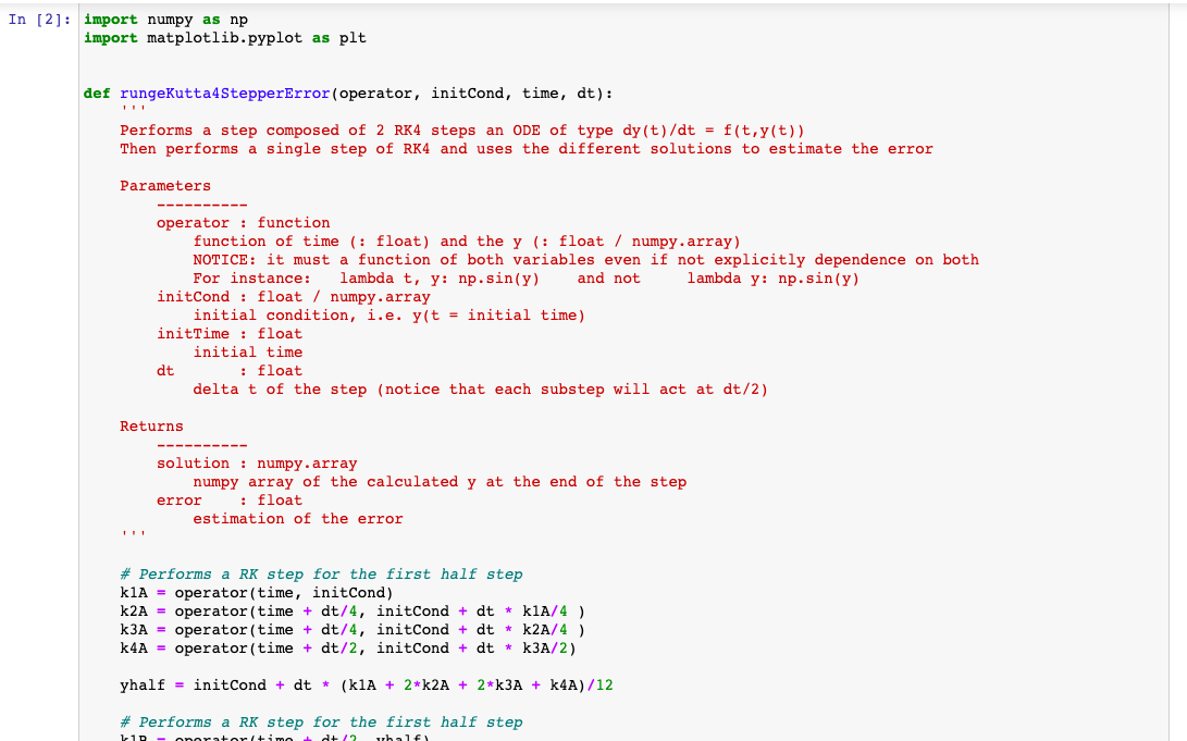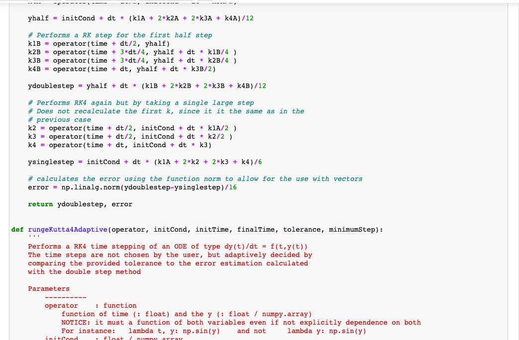Write a python function that takes as input: - mass of the mass \( 1 m_{1} \) in \( \mathrm{kg} \) - mass of the mass \( 2 m_{2} \) in \( \mathrm{kg} \) - length of the stick \( 1 L_{1} \) in \( m \) - length of the stick \( 2 L_{2} \) in \( \mathrm{m} \) - initial value of angle \( \theta_{1}\left(t=t_{0}\right) \) in rad - mass of the mass \( 1 m_{1} \) in \( \mathrm{kg} \) - mass of the mass \( 2 m_{2} \) in \( \mathrm{kg} \) - length of the stick \( 1 L_{1} \) in \( m \) - length of the stick \( 2 L_{2} \) in \( m \) - initial value of angle \( \theta_{1}\left(t=t_{0}\right) \) in rad - initial value of angle \( \theta_{2}\left(t=t_{0}\right) \) in rad - initial time - final time - tolerance on the error on the angles The python function should output: - times at which the two angles have been calculated - angle 1 at the above times - angle 2 at the above times The python function should calculate the above quantities using adaptive time step RK4 (with step doubling). After constructing the python function above, use its output to plot the trajectories: - angle 1 in dependence of time - angle 2 in dependence of time - xy position of mass 1 (you need to figure out how it depends on \( \theta_{1} \) ) - xy position of mass 2 (you need to figure out how it depends on \( \theta_{1} \) and \( \theta_{2} \) ) You do not need to make an animation, just a plot. You can create an animation for your own extra training, but it will not be graded. Below you find the definitions of the functions you will need (notice that they have been slightly modified from class to make sure that they work with this problem). There is no need to program them again, just use them. 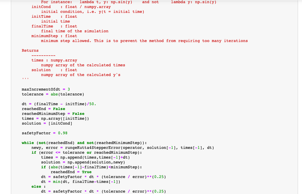import numpy as \( \mathrm{np} \) import matplotlib.pyplot as plt def rungekutta4stepperError(operator, initCond, time, dt): Performs a step composed of 2 RK 4 steps an ODE of type \( d y(t) / d t=f(t, y(t)) \) \[ d t=\text { safetyFactor } * d t * \text { (tolerance / error) } * \star(0.25) \] if \( d t< \) minimumStep: reachedMinimumStep = True return times, np.array(solution) Hints - Watch out, these are 2 second order ordinary differential equations, so you first need to transform them into 4 first order ODE. - Your solution, initial condition and operator that gives the derivatives are going to be in vectors. Decide which element of the verrestonds to what variable of the system and stick to that. 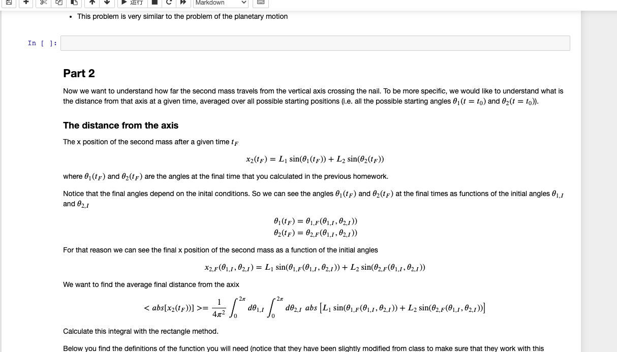- This problem is very similar to the problem of the planetary motion - This problem is very similar to the problem of the planetary motion Part 2 Now we want to understand how far the second mass travels from the vertical axis crossing the nail. To be more specific, we would like to understand what is the distance from that axis at a given time, averaged over all possible starting positions \( \left(i . e\right. \). all the possible starting angles \( \theta_{1}\left(t=t_{0}\right) \) and \( \theta_{2}\left(t=t_{0}\right) \) ). The distance from the axis The \( \mathrm{x} \) position of the second mass after a given time \( t_{F} \) \[ x_{2}\left(t_{F}\right)=L_{1} \sin \left(\theta_{1}\left(t_{F}\right)\right)+L_{2} \sin \left(\theta_{2}\left(t_{F}\right)\right) \] where \( \theta_{1}\left(t_{F}\right) \) and \( \theta_{2}\left(t_{F}\right) \) are the angles at the final time that you calculated in the previous homework. Notice that the final angles depend on the inital conditions. So we can see the angles \( \theta_{1}\left(t_{F}\right) \) and \( \theta_{2}\left(t_{F}\right) \) at the final times as functions of the initial angles \( \theta_{1, I} \) and \( \theta_{2, I} \) \[ \begin{array}{l} \left.\theta_{1}\left(t_{F}\right)=\theta_{1, F}\left(\theta_{1, I}, \theta_{2, I}\right)\right) \\ \left.\theta_{2}\left(t_{F}\right)=\theta_{2, F}\left(\theta_{1, I}, \theta_{2, I}\right)\right) \end{array} \] For that reason we can see the final \( \mathrm{x} \) position of the second mass as a function of the initial angles \[ x_{2, F}\left(\theta_{1, I}, \theta_{2, I}\right)=L_{1} \sin \left(\theta_{1, F}\left(\theta_{1, I}, \theta_{2, I}\right)\right)+L_{2} \sin \left(\theta_{2, F}\left(\theta_{1, I}, \theta_{2, I}\right)\right) \] We want to find the average final distance from the axix \[ \left.=\frac{1}{4 \pi^{2}} \int_{0}^{2 \pi} d \theta_{1, I} \int_{0}^{2 \pi} d \theta_{2, I} a b s\left[L_{1} \sin \left(\theta_{1, F}\left(\theta_{1, I}, \theta_{2, I}\right)\right)+L_{2} \sin \left(\theta_{2, F}\left(\theta_{1, I}, \theta_{2, I}\right)\right)\right] \] Calculate this integral with the rectangle method. 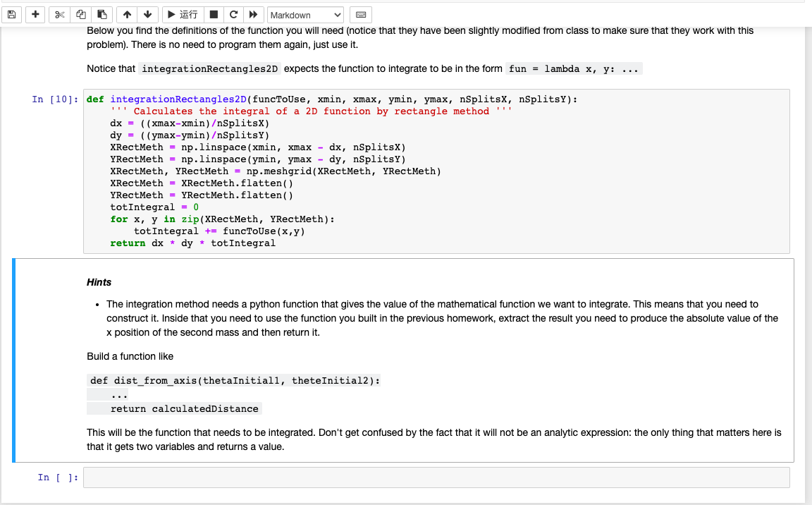Below you find the definitions of the function you will need (notice that they have been slightly modified from class to make sure that they work with this Below you find the definitions of the function you will need (notice that they have been slightly modified from class to make sure that they work with this problem). There is no need to program them again, just use it. Notice that integrationRectangles2D expects the function to integrate to be in the form fun \( =\operatorname{lambda} \mathrm{x}, \mathrm{y}: \ldots \) In [10]: def integrationRectangles2D(funcToUse, xmin, xmax, ymin, ymax, nSplitsX, nSplitsY): '' Calculates the integral of a 2D function by rectangle method ' ' \( \mathrm{dx}=((x \max -\mathrm{xmin}) / \mathrm{nSplits \textrm {X } )} \) \( d y=((y \max -y \min ) / \mathrm{nSplitsY}) \) XRectMeth \( =\mathrm{np} \).linspace \( (\mathrm{xmin} \), xmax \( -\mathrm{dx}, \mathrm{nSplitsX}) \) YRectMeth \( =\mathrm{np} \).linspace \( (\mathrm{ymin}, \mathrm{ymax}-\mathrm{dy}, \mathrm{nSplitsY}) \) XRectMeth, YRectMeth = np.meshgrid(XRectMeth, YRectMeth) XRectMeth \( = \) XRectMeth.flatten() YRectMeth \( = \) YRectMeth.flatten() totintegral \( =0 \) for \( x, y \) in zip(XRectMeth, YRectMeth): totIntegral += funcToUse \( (x, y) \) return \( \mathrm{dx} \) * \( \mathrm{dy} \) * totintegral Hints - The integration method needs a python function that gives the value of the mathematical function we want to integrate. This means that you need to construct it. Inside that you need to use the function you built in the previous homework, extract the result you need to produce the absolute value of the \( x \) position of the second mass and then return it. Build a function like def dist_from_axis(thetainitial1, theteInitial2): \( \quad \).. return calculatedDistance This will be the function that needs to be integrated. Don't get confused by the fact that it will not be an analytic expression: the only thing that matters here is that it gets two variables and returns a value.