(Solved): Consider the feedback control system shown in Figure Q.IV with a negative unit feedback. \( G_{p}(s ...

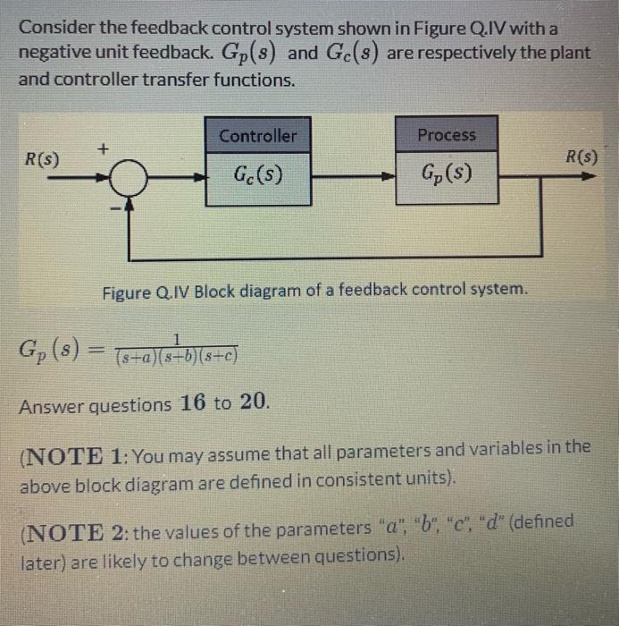
Consider the feedback control system shown in Figure Q.IV with a negative unit feedback. \( G_{p}(s) \) and \( G_{c}(s) \) are respectively the plant and controller transfer functions. Figure Q.IV Block diagram of a feedback control system. \[ G_{p}(s)=\frac{1}{(s+a)(s-b)(s+c)} \] Answer questions 16 to 20 (NOTE 1: You may assume that all parameters and variables in the above block diagram are defined in consistent units). (NOTE 2: the values of the parameters " \( a \) ", " \( b \) ", " \( c \) ". " \( d \) " (defined later) are likely to change between questions). 5 points Consider the controller transfer function as: \[ G_{c}(s)=\frac{K}{(s+d)} \] What are the angles between the positive direction of the real axis and the asymptotes of the root locus plot of the system? \( 45^{\circ} \) and \( 135^{\circ} \) None of the answer choices given \( 180^{\circ} \) \( 60^{\circ} \) and \( 180^{\circ} \) \( 90^{\circ} \) 5 points Consider the controlled system of Q16. Find the approximate distance between the origin of the \( s \)-plane and the point on the imaginary axis where the root loci cross the imaginary axis. 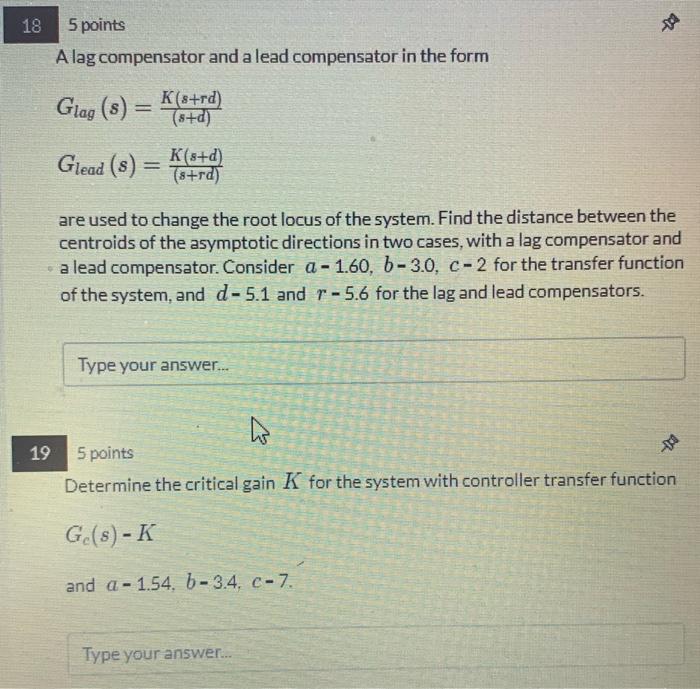Consider \( a-1.96, b-2.9, c-2 \), and \( d \) \( 4.7 \) A lag compensator and a lead compensator in the form \[ \begin{array}{l} G_{\text {lag }}(s)=\frac{K(s+r d)}{(s+d)} \\ G_{\text {lead }}(s)=\frac{K(s+d)}{(s+r d)} \end{array} \] are used to change the root locus of the system. Find the distance between the centroids of the asymptotic directions in two cases, with a lag compensator and a lead compensator. Consider \( a-1.60, b-3.0, c-2 \) for the transfer function of the system, and \( d-5.1 \) and \( r-5.6 \) for the lag and lead compensators. 5 points Determine the critical gain \( K \) for the system with controller transfer function \[ G_{c}(s)-K \] and \( a-1.54, b-3.4, c-7 \)