(Solved): Asap Fig. 16.9. Polynomial reduction of the 2-factor problem to the 1-factor problem \( G \) c ...

Asap

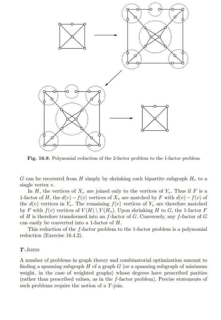
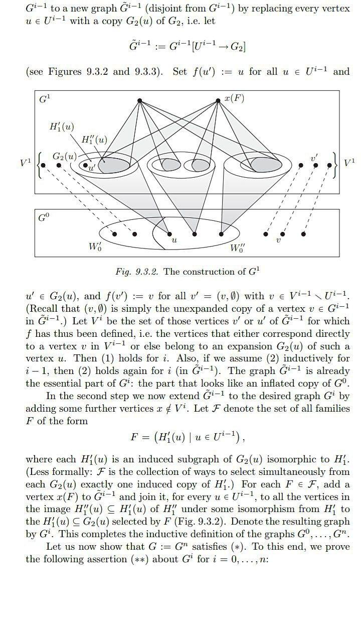
Fig. 16.9. Polynomial reduction of the 2-factor problem to the 1-factor problem \( G \) can be recovered from \( H \) simply by shrinking each bipartite subgraph \( H_{v} \) to a single vertex \( v \). In \( H \), the vertices of \( X_{v} \) are joined only to the vertices of \( Y_{v} \). Thus if \( F \) is a 1-factor of \( H \), the \( d(v)-f(v) \) vertices of \( X_{v} \) are matched by \( F \) with \( d(v)-f(v) \) of the \( d(v) \) vertices in \( Y_{v} \). The remaining \( f(v) \) vertices of \( Y_{v} \) are therefore matched by \( F \) with \( f(v) \) vertices of \( V(H) \backslash V\left(H_{v}\right) \). Upon shrinking \( H \) to \( G \), the 1-factor \( F \) of \( H \) is therefore transformed into an \( f \)-factor of \( G \). Conversely, any \( f \)-factor of \( G \) can easily be converted into a 1-factor of \( H \). This reduction of the \( f \)-factor problem to the 1-factor problem is a polynomial reduction (Exercise 16.4.2). T-JoINS A number of problems in graph theory and combinatorial optimization amount to finding a spanning subgraph \( H \) of a graph \( G \) (or a spanning subgraph of minimum weight, in the case of weighted graphs) whose degrees have prescribed parities (rather than prescribed values, as in the \( f \)-factor problem). Precise statements of such problems require the notion of a \( T \)-join. \( G^{i-1} \) to a new graph \( \tilde{G}^{i-1} \) (disjoint from \( G^{i-1} \) ) by replacing every vertex \( u \in U^{i-1} \) with a copy \( G_{2}(u) \) of \( G_{2} \), i.e. let \[ \tilde{G}^{i-1}:=G^{i-1}\left[U^{i-1} \rightarrow G_{2}\right] \] (see Figures 9.3.2 and 9.3.3). Set \( f\left(u^{\prime}\right):=u \) for all \( u \in U^{i-1} \) and Fig. 9.3.2. The construction of \( G^{1} \) \( u^{\prime} \in G_{2}(u) \), and \( f\left(v^{\prime}\right):=v \) for all \( v^{\prime}=(v, \emptyset) \) with \( v \in V^{i-1} \backslash U^{i-1} \). (Recall that \( (v, \emptyset) \) is simply the unexpanded copy of a vertex \( v \in G^{i-1} \) in \( \tilde{G}^{i-1} \).) Let \( V^{i} \) be the set of those vertices \( v^{\prime} \) or \( u^{\prime} \) of \( \tilde{G}^{i-1} \) for which \( f \) has thus been defined, i.e. the vertices that either correspond directly to a vertex \( v \) in \( V^{i-1} \) or else belong to an expansion \( G_{2}(u) \) of such a vertex \( u \). Then (1) holds for \( i \). Also, if we assume (2) inductively for \( i-1 \), then (2) holds again for \( i \) (in \( \tilde{G}^{i-1} \) ). The graph \( \tilde{G}^{i-1} \) is already the essential part of \( G^{i} \) : the part that looks like an inflated copy of \( G^{0} \). In the second step we now extend \( \tilde{G}^{i-1} \) to the desired graph \( G^{i} \) by adding some further vertices \( x \notin V^{i} \). Let \( \mathcal{F} \) denote the set of all families \( F \) of the form \[ F=\left(H_{1}^{\prime}(u) \mid u \in U^{i-1}\right), \] where each \( H_{1}^{\prime}(u) \) is an induced subgraph of \( G_{2}(u) \) isomorphic to \( H_{1}^{\prime} \). (Less formally: \( \mathcal{F} \) is the collection of ways to select simultaneously from each \( G_{2}(u) \) exactly one induced copy of \( H_{1}^{\prime} \).) For each \( F \in \mathcal{F} \), add a vertex \( x(F) \) to \( \tilde{G}^{i-1} \) and join it, for every \( u \in U^{i-1} \), to all the vertices in the image \( H_{1}^{\prime \prime}(u) \subseteq H_{1}^{\prime}(u) \) of \( H_{1}^{\prime \prime} \) under some isomorphism from \( H_{1}^{\prime} \) to the \( H_{1}^{\prime}(u) \subseteq G_{2}(u) \) selected by \( F \) (Fig. 9.3.2). Denote the resulting graph by \( G^{i} \). This completes the inductive definition of the graphs \( G^{0}, \ldots, G^{n} \). Let us now show that \( G:=G^{n} \) satisfies \( (*) \). To this end, we prove the following assertion \( (* *) \) about \( G^{i} \) for \( i=0, \ldots, n \) : the line-segment from \( f(x) \) to \( g(x) \) is always contained in \( A \). Then \( H(x, t)= \) \( (1-t) f(x)+\operatorname{tg}(x) \) is a homotopy from \( f \) to \( g \) (linear homotopy). It will turn out that many homotopies are constructed from linear homotopies. A set \( A \subset \mathbb{R}^{n} \) is star-shaped with respect to \( a_{0} \in A \) if for each \( a \in A \) the line-segment from \( a_{0} \) to \( a \) is contained in \( A \). If \( A \) is star-shaped, then \( H(a, t)= \) \( (1-t) a+t a_{0} \) is a null homotopy of the identity. Hence star-shaped sets are contractible. A set \( C \subset \mathbb{R}^{n} \) is convex if and only if it is star-shaped with respect to each of its points. Note: If \( A=\mathbb{R}^{n} \) and \( a_{0}=0 \), then each \( H_{t}, t<1 \), is a homeomorphism, and only in the very last moment is \( H_{1} \) constant! This is less mysterious, if we look at the paths \( t \mapsto H(x, t) \). The reader should now recall the notion of a quotient map (identification), its universal property, and the fact that the product of a quotient map by the identity of a locally compact space is again a quotient map (see (2.4.6)). (2.1.6) Proposition. Let \( p: X \rightarrow Y \) be a quotient map. Suppose \( H_{t}: Y \rightarrow Z \) is a family of set maps such that \( H_{t} \circ p \) is a homotopy. Then \( H_{t} \) is a homotopy.